Theory

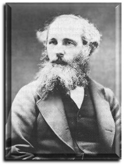
James Clerk Maxwell (1837-1879) gathered all prior knowledge in electromagnetics and summoned the whole theory of electromagnetics in four equations, called the Maxwell’s equations.

To evolve the Maxwell’s equations we start with the fundamental postulates of electrostatics and magnetostatics. These fundamental relations are considered laws of nature from which we can build the whole electromagnetic theory.

According to Helmholtz’s theorem, a vector field is determined to within an additive constant if both its divergence and its curl are specified everywhere [8]. From this an electrostatic model and a magnetostatic model are derived only by defining two fundamental vectors, the electric field intensity E and the magnetic flux density B, and then specifying their divergence and their curls as postulates. Written in their differential form we have for the electrostatic model the following two relations' [8]:

These are based on the electric field intensity vector, E, as the only fundamental field quantity in free space. Then to account for the effect of polarization in a medium the electric flux density, D, is defined by the constitutive relation:

where the permittivity e is a scalar (if the medium is linear and isotropic). Similarly for the magnetostatic model we have the following two relations, based on the magnetic flux density vector, B, as the fundamental field quantity:

where J is the current density. To account for the material here as well, we define another fundamental field quantity, the magnetic field intensity, H, and we get the following constitutive relation:

where m is the permeability of the medium. Using the constitutive relations we can rewrite the postulates and the relations derived is gathered in the following table:

Table 1 Fundamental Relations for Electrostatic and Magnetostatic Models (The Governing Equations)

*The Governing Equations*
*Electrostatic Model*
	Equation 13
	Equation 14
*Magnetostatic Model*
	Equation 15
	Equation 16

These equations must, however, be revised for calculation of time varying fields. The electrostatic model must be modified due to the observed fact that a time varying magnetic field gives rise to an electric field and vice versa and the magnetostatic model must be modified in order to be consistent with the equation of continuity.

The complete model for electromagnetic fields (Maxwell’s equations) is gathered in the following table (Table 2), where the integral forms of the equations are added [8]:

*Maxwell’s Equations*
*Faraday’s law*
	Equation 17
	Equation 18
*Ampère’s circuital law*
	Equation 19
	Equation 20
*Gauss’s law*
	Equation 21
	Equation 22
*No isolated magnetic charge*
	Equation 23
	Equation 24

We can see in Equation 17 that the electric field intensity vector

(Equation 13) is replaced with

according to Faraday’s law of electromagnetic induction [8]. In Equation 19, the term

is called displacement current density and its introduction was one of the major contributions by Maxwell. The displacement current density is necessary in order to make the equations consistent with the principle of conservation of charge in the time varying case.

There are many ways of solving and using these equations. One technique to make the solution of Maxwell’s equations easier, which we will use later, is to use potential functions. It is known that if a vector field is divergence less, then it can be expressed as the curl of another vector field. For instance since the divergence of B is zero,

, then B can be expressed as the curl of the vector field A:

where A is called the vector magnetic potential and it can be determined from the current distribution J:

Using the constitutive relations, Equation 9 and Equation 12, the magnetic field intensity H can then be calculated as:

The electric field intensity E can also be calculated using potential functions by introduction of the scalar electric potential V:

When both the vector magnetic potential A and the scalar electric potential V are known, the electric field intensity E is derived by:

It is however not necessary to calculate both the magnetic field intensity H and the electric field intensity E since they are related by the equation:

	Equation 6
	Equation 7

	Equation 10
	Equation 11

2 Maxwell’s Equations