Theory

Introduction to Electromagnetics

Maxwell's Equations

Near-Field and Far-Field

Transmission Line

Models

Scale modeling

References

Symbols and units

Constants

Mutual Impedance Between Wire Elements

3 Near-Field and Far-Field

In this chapter we will solve the Maxwell’s equations for a radiating wire and by analyzing the solution we will define the near-field and the far-field. The electromagnetic field radiating from a wire can be calculated by solving Maxwell’s equations for a short current element and then placing the current elements end-to-end.

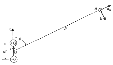
Figure 3 A small current element or an electric dipole.

To be able to derive the field of a conducting element acting as an electrical dipole, the current in the element is defined to flow along an axis z. This gives that the magnetic vector potential can be expressed as (see Equation 26):

Equation 31

where:

Equation 32

It is wise to use spherical coordinates when deriving the field of a small current element that can be approximated with a point source

Equation 33

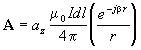
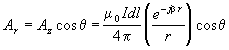
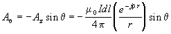
If A is then expressed in the form

Equation 34

it can apparently be divided into the spherical components:

	Equation 35
	Equation 36
	Equation 37

The intensity of the magnetic field is then (using Equation 27):

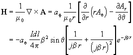Equation 38

According to Equation 30 above E can be determined when H is known:

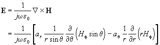Equation 39

Which results in:

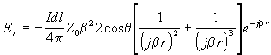	Equation 40
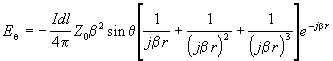	Equation 41
	Equation 42

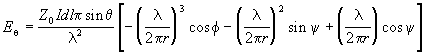
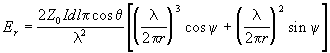
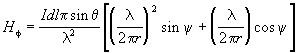
By rewriting those equations we can identify the wavelength and get the following equations in Table 3. A summation of the theory above states that:

If the length of one element is much less than a wavelength (dl << l ) and the element is considered as an oscillating dipole the electric and magnetic fields for one element can, with the use of some algebra, be expressed as:

Table 3 The electric and magnetic field equations for a small oscillating electric dipole

*Electric and Magnetic Field Equations for an Electric Dipole*
	Equation 43
	Equation 44
	Equation 45

where:

dl is the length of the current element
y is a short for (2p f/l )-w t
w is the radian frequency of the signal
t is the time (=1/f)
c is the speed of light (m/s)
Z₀ is the free space impedance (» 377 W )
I is the current in the element
q is the zenith angle to radial distance r
l is the wavelength of the signal
r is the distance from the element to the point of observation

Analyzing these equations (Equation 43 to Equation 45) we can divide the terms into three different basic terms:

one inverse distance term proportional to r^-1 which is called the radiation term. This term represents the flow of energy away from the wire.
one inverse square distance term proportional to r^-2 which is called the induction term and represents energy stored in the field during one quarter of a cycle and then returned to the antenna in the next.
and finally one inverse cube distance term proportional to r^-3 that is called the quasi stationary term, or the electrostatic field term, and results from the accumulation of charge at the ends of the element.

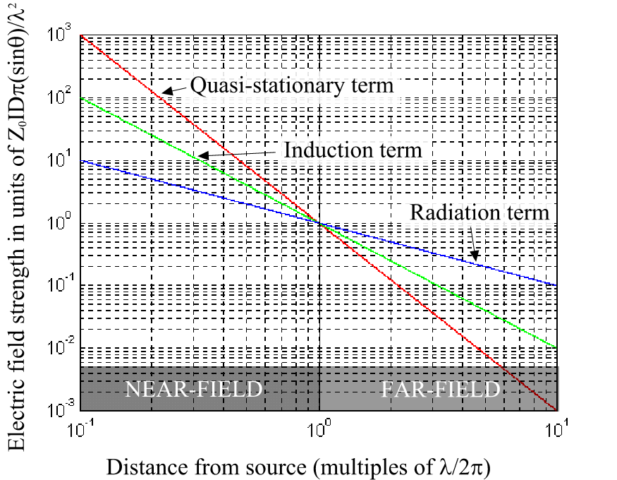
Figure 4 The significance of the different terms for the electric field strength

Notice that all these terms with the coefficients , and will all be equal (=1) at the distance . This distance is in this report said to be the boundary between near-field and far-field and the contributions from the radiation, induction and the electrostatic term are all of the same magnitude.

When r << only the first term in each equation is significant and will in this case mean that the wave impedance will be:

Equation 46

that is much greater than the free space impedance Z₀ i.e. we will have a high E-field and a low H-field. If the current element had been a current loop with a low circuit impedance instead of the high circuit-impedance of the current element, the first term, or the electrostatic term, in the first two equations (Equation 43 and Equation 44) would disappear and a similar equation would appear in Equation 45. In this case the wave impedance would be:

Equation 47

representing a high H-field and a low E-field in the near-field.

When r >> the last term proportional to r^-1 in Equation 43 and Equation 45 will dominate and the wave impedance will approach the free space impedance Z₀ = 377W . This is called the far-field or radiation field. The Eq and the Hf fields will then be in phase and orthogonal to each other producing plane waves. This is illustrated in Figure 5 below:

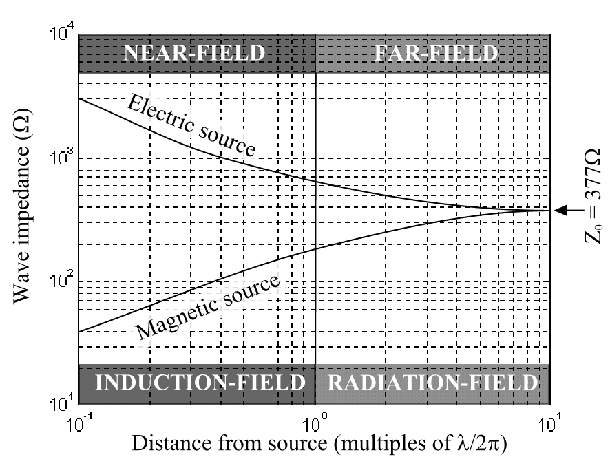
Figure 5 Wave impedance at different distances from either an electric source or a magnetic source

When such current elements are placed end-to-end to produce a model of a radiating wire, the charge at the ends of the elements will cancel and the term due to the electrostatic field (the one proportional to r^-3) will disappear. This is however only true with a constant current distribution on the line. With a varying current distribution the electrostatic fields will not cancel entirely. However, if the wire is divided into a sufficient number of segments per wavelength then this error will be small.

The length of telecommunication lines and the size of telecommunication systems are often greater than one wavelength, D ³ l . If the dimension of the field source D is greater than a wavelength the near-field/far-field boundary is said to be at the distance [5]:

Equation 48

At a shorter distance maxima and minima would appear due to interference caused by different distances to different parts of the source.

Previous: Maxwell's Equations | Next: Transmission Line